Generalizing to
a Population:
COMPLEX MODELS: More Than One
Independent Variable continued
 Multiple Linear Regression
model: numeric <= numeric1 numeric2...
+ interactions
example: weight <= height age height*age
 The
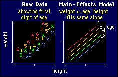
example shows weights and heights of a sample of people aged between 20 and 60.
Each person is represented by a number, which is the person's age rounded to the
nearest decade (2 = 15-24 years, 3 = 25-34 years, etc.). Look closely at the way
the numbers are distributed. What would you conclude about the effect of age on
weight, for any given height? Right! People get heavier as they get older.
Multiple linear regression is the model to use when you want to
look at data like these, consisting of two or more numeric
independent variables (height, age) and a numeric dependent variable
(weight). In this first example, the only effect of age is to produce
a uniform increase in weight, irrespective of height. It's just as
correct to say there is a uniform increase in weight with height,
irrespective of age. These interpretations come straight from the
model. Or you can look at the graphical interpretation and think
about the effect of age as altering the intercept of the
weight-height line in a uniform way. But what about when there's an
interaction?
Interpreting the Interaction Term
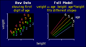
 As you can see, the effect of an interaction
is to make different slopes for different ages. The slopes change in a nice
linear way with increasing age, just as the intercepts did (and still do). In
the example, I've given older people a greater weight for a given height than
younger people, which is not necessarily realistic. Real data would certainly
not show such clear-cut effects of either height or weight, anyway.
It's one thing for me to show you a clear-cut example with colors
for the different ages. It's quite another matter for you to
interpret real data, without a colored graph. If you get a
substantial interaction with your data, I suggest you look at the
values of the parameters in the solution. Use them to work out how
your outcome variable is affected by a range of values of the
independent variables. That's the only way you will sort out what's
going on.
By the way, for publication you would not plot them as I have
shown here. In fact, generally you don't plot the data for linear
regressions, be they simple or multiple, unless the data show
interesting non-linear effects.
Paradoxically Insubstantial Effects
On the previous page
I pointed out how one independent variable can make another seem insubstantial
in an ANCOVA. The same is true here. It's important, so let's take an example.
Suppose you want to predict running-shoe size (dependent variable)
from an athlete's height and weight. These two variables are well
correlated, but let's assume the correlation is almost perfect. When
two variables have an almost perfect correlation, it means they
effectively measure the same thing, even if they are in different
units. Now let's put them both into the model. Will weight tell you
anything extra about shoe size, when height is already in the model?
No, because weight isn't measuring anything extra, so it won't be
substantial in the model. But hey, height won't be substantial with
weight in the model, for the same reason. So you have the bizarre
situation where neither effect is substantial, and yet both are
obviously substantial! If you didn't know about this phenomenon, you
might look at the p values for each effect in the model, see that
they are both greater than 0.05, and conclude that there is no
significant effect of either height or weight on shoe size.
The trick is to look at the p value for the whole model as well.
None of the effects might be significant, but the whole model will be
very significant. And you should always look at the main effects
individually, as simple linear regressions or correlations, before
you go to the multiple model. You'd find they were both
substantial/significant.
So in this example, would you use both independent variables to predict shoe
size? Not an easy question to answer. I'd look to see just how much bigger the
R2 gets with the second independent variable
in the model, regardless of its statistical significance. More on this, next.
Now for two important applications of multiple linear regression: stepwise
regression, and on the next page, polynomial
regression.
 Stepwise Regression
model: numeric <= numeric1 numeric2 numeric3...
example: competitive speed <= a
set of fitness-test variables
No figure is needed for this one. No interactions either,
thank goodness! Numeric1, numeric2, and so on are independent variables, and you
try to find the best ones for predicting your dependent variable.
An obvious example is where your dependent variable is some
measure of competitive performance, like running speed over 1500 m,
and your independent variables are the results of all sorts of
fitness tests for aerobic power, anaerobic power, and body
composition. What's the best way to combine the tests to predict
performance? An interesting and possibly useful question, because you
can use the answer for talent identification or team selection. (Why
not use the 1500-m times for that purpose? Hmmm...) Anyway, in
stepwise regression the computer program finds the lab test with the
highest correlation (R2) with
performance; it then tries each of the remaining variables (fitness
tests) in a multiple linear regression until it finds the two
variables with the highest R2; then
it tries all of them again until it finds the three variables
with the highest R2, and so on. The
overall R2 gets bigger as you add
in more variables. Ideally of course, you hope to explain 100% of the
variance.
Now, even random numbers will explain some of the variance,
because you never get exactly zero for a correlation with real
numbers. So you need an arbitrary point at which to cut off any
further variables from entering the analysis. It's done with the p
value, and the default value is 0.15. When a variable enters the
model with a p value >0.15, the stepwise procedure halts. You'd
hardly call a p value of 0.15 significant, but it's OK if you're
using stepwise regression as an exploratory tool to identify the
potentially important predictors.
The question of what variables you finally include for your
prediction equation is not just a matter of the p values, though. You
should be looking at the R2 and
deciding whether the last few variables in the stepwise analysis add
anything worthwhile, regardless of their significance. If the sample
size isn't as big as it ought to be, there's a good chance that the
last few variables will contribute substantially to the R2, and yet not be statistically significant.
You should still use them, but knowing that their real contributions
could be quite a bit different.
OK, what is a worthwhile increase in the R2 as each variable enters the model? Take the
square root of the total R2 after
each variable has entered, then interpret the resulting correlations
using the scale of magnitudes. If the
correlations are in the moderate-large range, an increase of 0.1 or
more is worthwhile. If the correlation is in the very large to almost
perfect range, then smaller increases (0.05 or even less) are
worthwhile, as I explain later.
Finally, a warning! If two independent variables are highly
correlated, only one will end up in the model with a stepwise
analysis, even though either can be regarded as predictors.
Go back up this page for the reason. And as
discussed in the previous paragraph, the decision to keep both in the
model depends on the R.
Go to: Next · Previous · Contents · Search
· Home
webmaster=AT=newstats.org
Last updated 10 Dec 00
 As you can see, the effect of an interaction
is to make different slopes for different ages. The slopes change in a nice
linear way with increasing age, just as the intercepts did (and still do). In
the example, I've given older people a greater weight for a given height than
younger people, which is not necessarily realistic. Real data would certainly
not show such clear-cut effects of either height or weight, anyway.
 The
example shows weights and heights of a sample of people aged between 20 and 60.
Each person is represented by a number, which is the person's age rounded to the
nearest decade (2 = 15-24 years, 3 = 25-34 years, etc.). Look closely at the way
the numbers are distributed. What would you conclude about the effect of age on
weight, for any given height? Right! People get heavier as they get older.