|
A New View of Statistics | |

/*
Fitting polynomials to repeated measures data.
(Use polynomials only if it's appropriate to fit curves.)
Example for one within-subject effect (time), with six equally spaced
levels, plus one between effect (grp) to represent groups doing
overload and control training.
*/

options linesize=78;
options pagesize=32;

/*
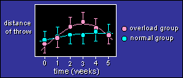
Generates data for 20 athletes in each group:
    true means=60, 62 (at time=0);
    between SDs=8 (excluding within SD);
    within SDs=3.
The mean increases by 0.2 at each retest in each group, to simulate a
linear learning effect.
A quadratic effect peaking at time=3 is added to the overload group.
The normal group has a smaller quadratic effect, peaking at time=4.
Try 200 athletes in each group if you want to see these effects clearly.
*/

data dat1;
grp="overload";
do athlete=1 to 20;
  true=60+8*rannor(0);
  do time=0 to 5;
    distance=true+0.2*time+0.7*(9-(time-3)**2)+3*rannor(0);
    output;
  end;
end;
grp="normal";
do athlete=21 to 40;
  true=62+8*rannor(0);
  do time=0 to 5;
    distance=true+0.2*time+0.1*(16-(time-4)**2)+3*rannor(0);
    output;
  end;
end;

*checks means and SDs of data;
proc sort;
by grp time;

proc means noprint;
var distance;
output mean=meandist std=sddist n=n;
by grp time;

proc print;
var grp time n meandist sddist;
format _numeric_ 4.0;
title "Means and SDs for each time in each group";

*plots means of data;
proc plot;
plot meandist*time=grp;
title "Means at each time point for each group";
run;

/*
*first time through, with time as a classification effect;
*no need to specify time explicitly as the repeated effect;
proc mixed data=dat1;
class athlete grp time;
model distance=grp time grp*time;
repeated /subject=athlete r rcorr type=un;
title "First pass, unstructured covariance matrix, time as a class effect";
run;
*/

/*
Second time through, as a cubic (third-order polynomial).
Do NOT specify time explicitly as a repeated effect.
proc mixed data=dat1;
class athlete grp;
model distance=grp time grp*time time*time grp*time*time
   time*time*time grp*time*time*time;
repeated /subject=athlete rcorr type=cs;
title "Second pass, to check whether need cubic terms";
run;
*/

/*
Third time through, full analysis as a quadratic (second-order polynomial).
Do NOT specify time explicitly as a repeated effect.
The estimates shown compare changes in the two groups relative to baseline
(time=0).  With your own data, make sure time=0 for your baseline point;
the estimates are a bit tricky to specify otherwise.  (See the example
for baseline at x=1.)
You can also compare the contributions of linear and quadratic terms
by looking at the coefficients in the solution.  It's easier to interpret
these coefficients if you make your time axis go from -1 to +1.
*/
proc mixed data=dat1 covtest cl;
class athlete grp;
model distance=grp time grp*time time*time grp*time*time /solution cl;
repeated /subject=athlete r rcorr type=cs;
estimate 'diff at x=1' grp*time -1 1 grp*time*time -1 1/cl;
estimate 'diff at x=2' grp*time -2 2 grp*time*time -4 4/cl;
estimate 'diff at x=3' grp*time -3 3 grp*time*time -9 9/cl;
estimate 'diff at x=4' grp*time -4 4 grp*time*time -16 16/cl;
estimate 'diff at x=5' grp*time -5 5 grp*time*time -25 25/cl;
*example comparing changes relative to a baseline at x=1;
estimate 'diff at x=2 vs x=1' grp*time -1 1 grp*time*time -3 3/cl;
estimate 'diff at x=3 vs x=1' grp*time -2 2 grp*time*time -8 8/cl;
*etc!;
title "Third pass, polynomial of order 2, with compound symmetry";
run;

/*
Compare the estimates and width of confidence intervals for the
above with those of the following more usual analysis:
*/
proc mixed data=dat1;
class athlete grp time;
model distance=grp time grp*time;
repeated /subject=athlete rcorr type=cs;
estimate 'overload-normal 1-0' grp*time 1 -1 0 0 0 0  -1 1 0 0 0 0/cl;
estimate 'overload-normal 2-0' grp*time 1 0 -1 0 0 0  -1 0 1 0 0 0/cl;
estimate 'overload-normal 3-0' grp*time 1 0 0 -1 0 0  -1 0 0 1 0 0/cl;
estimate 'overload-normal 4-0' grp*time 1 0 0 0 -1 0  -1 0 0 0 1 0/cl;
estimate 'overload-normal 5-0' grp*time 1 0 0 0 0 -1  -1 0 0 0 0 1/cl;
*the comparisons for baseline at time=1 are easy with this analysis;
estimate 'overload-normal 2-1' grp*time 0 1 -1 0 0 0  0 -1 1 0 0 0/cl;
estimate 'overload-normal 3-1' grp*time 0 0 1 -1 0 0  0 0 -1 1 0 0/cl;
*etc!;
title "The less powerful, more usual way";
run;
Go to: Previous · Contents · Search
· Home
resources=AT=sportsci.org · webmaster=AT=sportsci.org · Sportsci Homepage · Copyright
©1997
Last updated 13 May 98