Generalizing to
a Population:
REPEATED-MEASURES
MODELS
continued
 Proc Mixed for
Repeated Measures
On this page I introduce several examples of repeated-measures data,
and I provide programs to analyze them using Proc Mixed in the Statistical Analysis
System (SAS). Proc Mixed uses mixed modeling,
a concept I have already introduced and which I will explain here in more detail
soon. I will also explain covariance matrices. Meanwhile, here are some general
remarks about the examples and the programs, followed by specific remarks for
each example and links to the programs.
It's more than five years since I wrote these pages and the SAS programs!
My approach has become more sophisticated during that time, but I haven't had
a chance to update things here yet. If you are running SAS and would like advice
and/or copies of my recent programs, contact me.
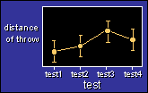 The data in each
example are for athletes tested on several occasions to determine the
distance they can throw an object, such as a javelin. (The figure
shows the simplest example.) In each example, the program creates a
sample of athletes drawn randomly from a population with a normal
distribution of throwing ability. Next, the program generates
normally-distributed within-subject random variation, which is simply
the variation in performance that each subject experiences between
tests. It then adds a change or changes in performance between some
tests, for example changes resulting from a training program. Finally
it uses Proc Mixed to analyze the data.
If you re-run any of these programs, the random variation between
and within subjects will produce a slightly different outcome, so the
data may not look exactly like what's in the figure accompanying each
example. It's the same as repeating the study with a different sample
of subjects. Try it and see, then play with the sample size, the
between- and within-subject variation, and the magnitude of the
change or changes in performance.
The main aim of the analysis is to calculate the changes in
performance between tests, and the confidence limits or p values for
the changes. Calculating the changes is usually easy: you just
subtract the mean of one or more tests from the mean of one or more
other tests. Calculating confidence intervals or p values is the hard
part. That's when you need a procedure like Proc Mixed or analysis of
variance. The procedure can also output the changes in performance,
to save you doing it on a spreadsheet.
Here are the examples:
More to come soon!
To analyze your own data, you will need to get help from someone
who knows how to set up a link from the SAS program to the data file
on your computer. That means adding a filename statement that
links to a data step containing an infile statement. I might
provide examples of that soon, too.
Simple
Repeated-Measures
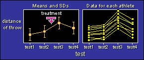
The figure shows data for a single group of subjects who
were tested four times. A treatment between test2 and test3 (for
example, supplementing for a week with a potentially ergogenic
nutritional like creatine) seems to have produced an increase in the
distance of the throw.

As noted above, the aim of the analysis is to calculate the mean
increase in the distance of the throw between the tests, and its
confidence limits or p value.
The data for each athlete show the kind of consistency of
performance you expect when there are no problems with sphericity, as
I discussed on the page devoted to three
or more tests and no between-subjects effect. In the accompanying
program, the analysis with an unstructured
covariance matrix serves as a check for such problems. If there
aren't any (and I didn't deliberately generate any), you use a
covariance matrix with compound symmetry, as shown in the program. It
won't make much sense until I provide a full explanation. Soon.
Adding
a Control Group
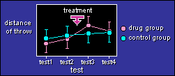
The data are the same as above, but this time there is a
control group who don't get any special treatment between test2 and
test3. The treatment could be something like a week of supplementing
with creatine (the drug group) or an inactive substance (the control
group).

Again, the aim of the analysis is to determine the confidence
limits for the increase, but this time it's the increase in the drug
group relative to (minus) the increase in the control group. Make
sure you understand the concepts on the pages devoted to
two trials plus a between-subjects
effect and three or more trials
plus a between-subjects effect before you try the
SAS program.
Fitting
Polynomials
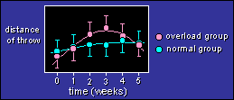
The figure shows data for two groups of athletes. After a
baseline test at time=0, one group did overload training, while the
other group continued with normal training.

The aim of the analysis is to compare the enhancement in the
overload group with that of the normal group at various times. You
can also compare the linear and quadratic components of the trends
between the groups. I'll add lots more on this topic soon.
See the earlier section on
polynomial contrasts before
you try the SAS program.
Individual Differences, and
Covariates
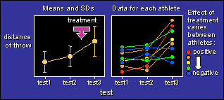
When different subjects have a different response to a treatment, we
say that there are individual differences in the response. I
first touched on this possibility when I dealt with repeated measures
with three or more trials and no control
group. Here I've limited it to three trials only, but I have
included a control group (not shown in the figure). In this example,
a treatment between test2 and test3 has produced an overall increase
in distance of a throw, but individual athletes differ widely in
their response to the treatment.

The aim of the analysis is...
- To estimate the overall effect of the treatment. That's
usually the change in the mean between test2 and test3. In the
example, the distance of the throw is increased by 3 m following
the treatment.
- To estimate the variability in the change in the mean between
test2 and test3. That represents the individual differences, and
it's best expressed as a standard deviation. In the example, the
standard deviation is 2 m. The increase in distance is therefore 3
± 2 m, which means that typical enhancements for individual
athletes (to the nearest meter) might be 2, 4, 3, 0, -1, 3, 6...
- Researchers sometimes calculate the standard deviation for
the difference between test3 and test2. This standard deviation
includes within-subject variation, so it is always larger than
the true measure of individual differences.
- To account for the individual differences with a subject
characteristic, such as age or percent of type 1 muscle fibers. In
the example, the ± 2 m is attributed entirely to another
variable, such that a change in that variable of one unit produces
a change in the throw of 2 m.
- To calculate the confidence limits for all of the above. For
example, the confidence limits for the 3 m might be 1 to 5 m, and
the confidence limits for the 2 m might be 0 to 5 m.
The SAS program generates data
for the treatment group, first without individual differences between
test2 and test3, then with them. It also generates the data for a
control group who have no shifts in the mean and no individual
differences between test2 and test3. The analysis includes
test1-test2 comparisons too.
This analysis is difficult, so I have included the
output of the program and
annotated it a little. Here's a summary of the output:
When there are no individual differences in the treatment group,
the change in performance between test2 and test3 is 2.7 ± 0.3
units (mean ± SD); the 95% confidence limits for the mean are
1.6 and 3.8; the 95% confidence limits for the SD are -1.1 and 1.2.
With individual differences present, the change in performance
between test2 and test3 is 2.5 ± 2.0 units (mean ± SD); the
95% confidence limits for the mean are 0.9 and 4.1; those for the SD
are 1.3 and 4.4.
With individual differences present, and with a covariate that
explains them included in the analysis, the change in performance
between test2 and test3 is 2.7 ± 0.3 units (mean ± SD); the
95% confidence limits for the mean are 1.5 and 3.9; those for the SD
are -1.1 and 1.2. The value of the covariate is 1.8 units of throwing
performance per unit of covariate; its 95% confidence limits are 0.5
and 3.2.
Go to: Next · Previous · Contents · Search
· Home
editor
Last updated 2 Nov 03
 The data in each
example are for athletes tested on several occasions to determine the
distance they can throw an object, such as a javelin. (The figure
shows the simplest example.) In each example, the program creates a
sample of athletes drawn randomly from a population with a normal
distribution of throwing ability. Next, the program generates
normally-distributed within-subject random variation, which is simply
the variation in performance that each subject experiences between
tests. It then adds a change or changes in performance between some
tests, for example changes resulting from a training program. Finally
it uses Proc Mixed to analyze the data.